IUSACO
2022-06-05 Sun
Input and Output
#include <cstdio>
using namespace std;
int main() {
    freopen("template.in", "r", stdin);
    freopen("template.out", "w", stdout);
}- When using C++, arrays should be declared globally, or initialized to zeros if declared locally to avoid garbage values.
- 32bit int: \(\pm 2\times10^{9}\) v/s 64bit int: \(\pm 9\times 10^{18}\)
Complexity and algorithm analysis
- Elementary mathematical calculation: O(1)
- Unordered set/map: O(1) per operation
- Binary Search: O(log n)
- Ordered set/map or Priority Queue: O(log n) per operation
- Prime factorization or primality check for int: \(O(\sqrt{n})\)
- Reading n inputs: O(n)
- Iterating through n element array: O(n)
- Sorting: Usually O(n log n) for
std::sort() - Iterating through all subsets of size k of input elements: O(\(n^{k}\) ), for triplets O(\(n^{3}\))
- Iterating through all subsets: O(\(2^{n}\))
- Iterating through all permutations: O(n!)
Built-in Data Structures
Data Structure determines how data is stored, each supports some operations efficiently. In following discussion, desired data type is put between <>. Most std structures support size() and empty() methods.
Iterators
Allows for traversal of a container with the help of a pointer.
for (vector<int>::iterator it = myvector.begin(); it != myvector.end(); ++it) {
    cout << *it; //prints the values in the vector using the pointer
}
Alternate way to achieve the same with a for-each loop and auto.
for(auto element : v){
    cout << element; // prints values in vector
}
Dynamic Arrays
Addition and deletion at the end in O(1) time and in the middle in O(n) time.
vector<int> v;
for(int i = 1; i <= 10; i++){
    v.push_back(i); // stores 1 to 10 in a dynamic array
}
Vectors can be made static sized by initializing it with a size, vector<int> v(30);. They also support an v.erase() operation. A dynamic array can be sorted (default ascending) by sort(v.begin(), v.end()).
Stacks and Queues
Stacks: LIFO with operations push (add at end), pop (remove at end) and top (show end) all of which are O(1). Declared as stack<int> s.
Queues: FIFO with operations push (add in front), pop (remove at end) and front (show end) in O(1).
Deques: Combination of a stack and a queue supporting insertion and deletion from both front and end. Operations are aptly named as push_back, push_font, pop_back and pop_front.
Priority Queues: Supports insertion of elements and deletion and retrieval of element with highest priority in O(log n) where priority is based on a comparator function (highest element in front). Has push (add at end), pop (remove at end) and top (show end) operations and is declared as priority_queue<int> pq;.
Sets
A set is a collection of objects having no duplicates.
Unordered Sets: Work by hashing that is, assigning a unique code to every object allowing for insert, erase and count (set contains element then 1 else 0) in O(1). Traversal is pointless. Declared as unordered_set<int> s.
for(int element : s){
    cout << element << " "; // iterating through a set, arbitrary order
}
Ordered Sets: Insertion, deletion and search needs O(log n) time. Has additional operations begin() (iterator to lowest element), end(), lower_bound() (iterator to least element ≥ some k) and upper_bound().
Multisets: A sorted set allowing multiple copies of same element, whose count operation returns the number of times an element is present in set. Time complexity of this operation is O(log n + f) where log n factor searches for element and f factor iterates through sorted set to get count. Declared as multiset<int> ms.
Maps
A map is a set of ordered pairs called key and value where keys must be unique but values can be repeated. Supported operations are addition and removal of key-value pair and retrieval of values for a given key. Unordered maps perform aforementioned methods in O(1) whereas for ordered maps it’s O(log n), sorted in order of key.
Unordered Maps: In map m, m[key] = value operator assigns value to a key and places the pair on the map, m[key] returns value associated with the key, count(key) checks for existence of key in the map and erase(it) removes pair associated with a key or iterator. Declared as unordered_map<int, int> m.
Ordered Maps: Supports additional operations lower_bound and upper_bound which return iterators pointing to lowest entry not less than/ strictly greater than a specified key.
map<int, int> m; // [(3,5); (11,4)]
m[10] = 491; // [(3,5); (10,491); (11,4)]
cout << m.lower_bound(10)->first << " " << m.lower_bound(10)->second << "\n";
// 10 491
cout << m.upper_bound(10)->first << " " << m.upper_bound(10)->second << "\n";
// 11 4
m.erase(11); // [(3,5); (10,491)]
Elementary Techniques
Simulation
Simulation refers to the act of doing precisely what the problem statement states and nothing else; essentially simulating it.
Complete Search
Brute forcing through all the possible cases in solution space to arrive at the solution. To iterate through all permutations of a list:
do {
    check(v); // process or check the current permutation for validity
} while(next_permutation(v.begin(), v.end()));
Sorting and Comparators
C++ has built-in function for sorting in ascending order: std::sort(arr, arr+N) or for a vector sort(v.begin(), v.end()). For sorting in a self-defined order, one must use a custom comparator.
Greedy Algorithms
Algorithms that select the most optimal choice at each step, instead of looking at the solution space as a whole. Usually in a greedy algorithm, there is a heuristic or value function that determines which choice is considered most optimal. The choice of the greedy algorithm matters too, for example in a scheduling problem choosing earliest starting next event would be incorrect, instead one should go for earliest ending next event because that would give one more choices for future events.
Greedy won’t work in all scenarios though, for example in the fairly popular coin change problem, if the denominations are {1,3,4} then greedy solution would be {4,1,1} but the correct least amount of coins would be two {3,3}. Similarly it cannot work for the knapsack problem which is solved using Dynamic Programming.
Graph Theory
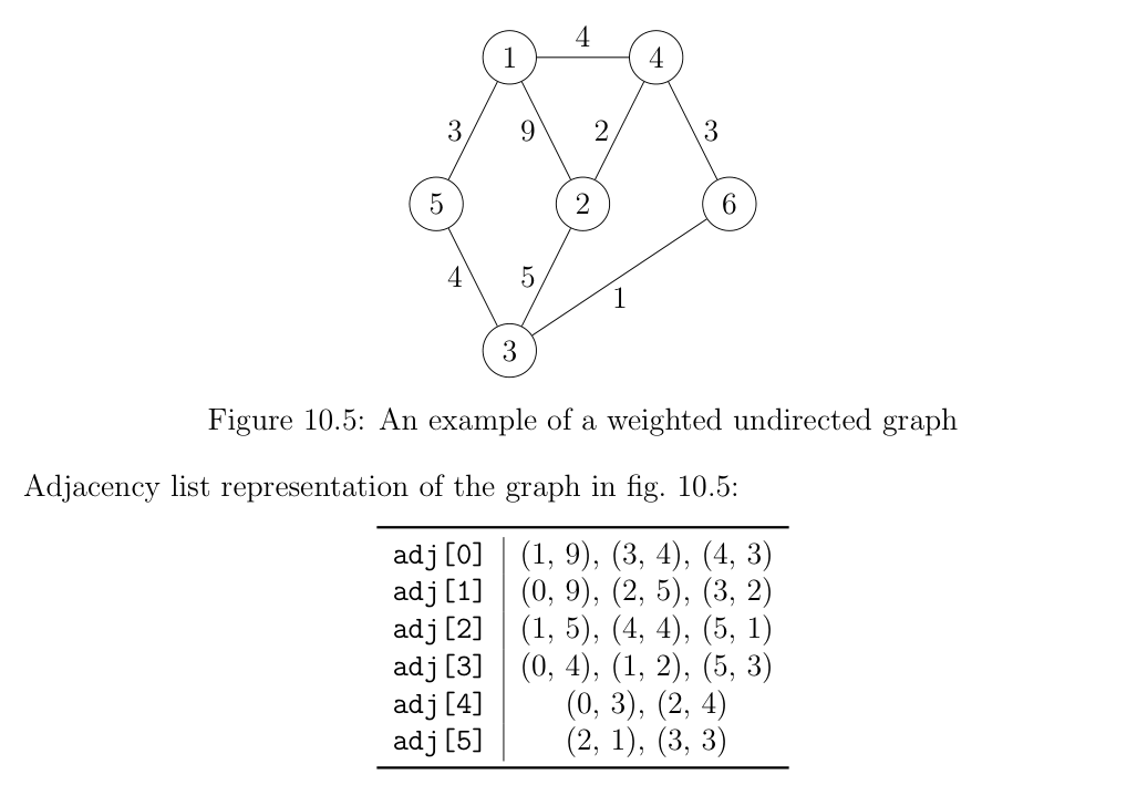
Representation
Graphs (N vertices and M edges) are usually given in the format: N M followed by the M edges each showing the connecting vertices. One thing to note is that a graph should be stored globally and statically, for access outside the main method. A graph can be represented in three ways:
Adjacency List
For using DFS, BFS, Dijkstra or other single-source traversal algorithms, it’s the preferred way of storing graphs. In it, an array of length N of lists is maintained.
 They take up
 O(M+N) space but allow for easy traversal among the neighbors of a vertex. Often, there’s a need to maintain a visited array.
int n, m;
vector<int> adj[MAXN];
bool visited[MAXN];

int main(){
    cin >> n >> m;
    for(int i = 0; i < m; i++){
        int a, b;
        cin >> a >> b;
        a--; b--; // subtract 1 for vertex since array is zero-indexed
        adj[a].push_back(b);
        adj[b].push_back(a); // omit for directed graph
    }
}

// For a weighted graph:
struct Edge {
    int to, weight;
    Edge(int dest, int w):
    to(dest), weight(w)
    {
    }
}
Adjacency Matrix
This is an N x N 2D array that stores for each pair of indices(a,b) whether an edge exists between them or not. Primarily used for Floyd-Warshall Algorithm.
int n, m;
int adj[MAXN][MAXN];

int main(){
    cin >> n >> m;
    for(int i = 0; i < m; i++){
        int a, b;
        cin >> a >> b;
        a--; b--;
        adj[a][b] = 1; // or w for weighted graph
        adj[b][a] = 1; // ignore this if directed
    }
}
Edge List
Usually used for weighted undirected graphs when sorting the edges by weight is needed (DSU). Its simply a single list of all edges (a, b, w) where a and b are the vertices and w is the weight of connecting edge. Each edge is added only oncce.
struct Edge{
    int a, b, w;
    Edge(int start, int end, int weight):
    a(start), b(end), w(weight)
    {
    }
    bool operator<(const Edge & e)
    const{
        return w < e.w; // ascending weight sort
    }
};

int n, m;
vector<Edge> edges;

int main(){
    cin >> n >> m;
    for(int i = 0; i < m; i++){
        int a, b, w;
        cin >> a >> b >> w;
        a--; b--;
        edges.push_back(Edge(a, b, w)); // add edge to list
    }
    sort(edges.begin(), edges.end());
}
Traversal
Breadth-First Search (BFS)
Visits nodes in order of distance away from the starting node; first visit nodes that are one edge away then those that are two edges away and so on. It can be used for finding the distance from a starting node to all nodes in an unweighted graph.
void bfs(int start){
    const int total_nodes = n;
    memset(dist, -1, sizeof dist); // fill distance array with -1s
    queue<int> q;
    dist[start] = 0;
    q.push(start);
    int seen = 1;
    while(!q.empty()){
        int v = q.front();
        q.pop();
        for(int e: adj[v]){
            if(dist[e] == -1){
                dist[e] = dist[v] + 1;
                 // see: https://observablehq.com/@yurivish/efficient-graph-search
                if(++seen == total_nodes) break;
                q.push(e);
            }
        }
    }
}
Once BFS finishes, the array dist contains the distances from the start node to each node.
Depth-First Search (DFS)
Continues down a single path as far as possible until it has no more vertices to visit along that path, then backtracks and finds more vertices to visit.
void dfs(int node){
    visited[node] = true;
    for(int next : adj[node]){
        if(!visited[next]){
            dfs(next);
        }
    }
}
If stack overflows are encountered with recursive DFS, it can be implemented iteravely by storing nodes in the BFS implementation on a stack instead of a queue.
Floodfill
Its DFS but on a grid and the aim is to find the connected component of all the connected cells with the same number. As opposed to an explicit graph where the edges are given, a grid is an implicit graph where the neighbours are nodes adjacent in the four directions.
When doing floodfill, an N x M array of bools visited is maintained and a global variable for the size of currently visiting component. The search function is called recursively from squares on all four sides of the current one.
int grid[MAXN][MAXM];
int n, m;
bool visited[MAXN][MAXM];
int currentCompSize = 0;

void floodfill(int r, int c, int color){
    if(r < 0 || r >= n || c < 0 || c >= m) return; // outside grid
    if(grid[r][c] != color) return; // wrong color
    if(visited[r][c]) return; // already visited

    visited[r][c] = true; // mark current sq as visited
    currentCompSize++;
    // recursively call floodfill for neighbour sqs
    floodfill(r, c+1, color);
    floodfill(r, c-1, color);
    floodfill(r-1, c, color);
    floodfill(r+1, c, color);
}

int main(){
    /*
     * additional stuff here
     */
    for(int i = 0; i < n; i++){
        for(int j = 0; j < m; j++){
            if(!visited[i][j]){
                currentCompSize = 0;
                floodfill(i, j, grid[i][j]);
            }
        }
    }
}
Disjoint-Set Union Data Structure
It supports two operations:
- Add an edge between two nodes
- Check if two nodes are connected
For this, the sets are stored as trees; initially each node is its own set then the sets are combined when an edge is added between two nodes.
int parent[MAXN]; // store root of each set

void initialize(int N){
    for(int i = 0; i < N; i++)
        parent[i] = i;      // initially, root of each set is node itself
}

int find(int x){            // find root of set of x
    if(x == parent[x])
        return x;           // if x is its parent, it is the root
    else
        return find(parent[x]);
}

void union(int a, int b){   // merge sets of a and b
    int c = find(a);        // find a's root
    int d = find(b);        // find b's root
    if (c != d)
        parent[d] = c;      // merge sets by setting parent of d to c
}
The naive recursive implementation of find can be improved from O(nm) by path compression; the idea being reassignment of nodes on recursive calls to find to prevent formation of long chains and the runtime becomes O(n log n).
int find(int x){
    if(x == parent[x])
        return x;
    else
        return parent[x] = find(parent[x]);
}
Miscellaneous
- DAGs (Directed Acyclic graphs) by virtue of not having any cycles allows them to have an ordering of nodes such that for any edge from u to v, u appears before v (topological sorting).
- Bipartite graph is such that each node can only be colored by 2 colors such that no adjacent nodes share the same colour. A graph is bipartite iff there are no cycles of odd length. A modified BFS can be use to check whether a graph is bipartite or not.
More Techniques
Prefix Sums
To process queries to find the sum of elements between two indices in a list, prefix sum is useful. Using 1-index in the array is beneficial i.e. assigning arr[0] = 0 and hence prefix[0] = 0.
\(prefix[k] = \sum_{i=1}^{k}arr[i] = prefix[k-1] + arr[k]\)
For processing Q queries consisting on an array of N elements, the complexity is O(N+Q).
TODO: DP, 2D prefix sum as 1-D only
Binary Search
Basic Number Theory
Prime factorization of a number is computed by this algorithm in \(O(\sqrt{n})\):
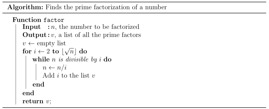
| i | n | v |
|---|---|---|
| 2 | 252 | {} |
| 2 | 126 | {2} |
| 2 | 63 | {2,2} |
| 3 | 21 | {2,2,3} |
| 3 | 7 | {2,2,3,3} |
| 7 | 1 | {2,2,3,3,7} |
GCD using Euclidean Algorithm in O(log min(a,b)):
int gcd(int a, int b){
    if(!b) return a;
    return gcd(b, a % b);
}
LCM can be computed using GCD by \(\frac{a \times b}{gcd(a,b)}\)
Modular Arithmetic is useful for dealing with overflows by taking remainders:
\[\begin{align*} (a \pm b)\mod m &= (a\mod m \pm b\mod m)\mod m \\ (a \times b)\mod m &= ((a\mod m) \times (b\mod m))\mod m \\ a^{b}\mod m &= (a\mod m)^{b}\mod m \end{align*}\]
Additional Topics
- Two Pointers
Iterate across an array that track the start and end of an interval or values in a sorted array. Both pointers are monotonic i.e. start at one end of array and move in only one direction.